• Products
    • Sage Intelligence Reporting
      • Enrolment
    • Velixo
      • Enrolment
        • Velixo for Acumatica
        • Velixo for Sage Intacct
  • Services
    • Consulting
    • Training
    • Development
  • Support
    • Support Overview
    • Create Support Ticket
    • Book A Session
    • Knowledgebase
  • About
    • About Us
  • Contact
  • Products
    • Sage Intelligence Reporting
      • Enrolment
    • Velixo
      • Enrolment
        • Velixo for Acumatica
        • Velixo for Sage Intacct
  • Services
    • Consulting
    • Training
    • Development
  • Support
    • Support Overview
    • Create Support Ticket
    • Book A Session
    • Knowledgebase
  • About
    • About Us
  • Contact
Quick Support
Book Demo

How to use a slicer instead of a drop-down list in Excel

By admin on April 11, 2018April 19, 2019

Selecting data from a drop-down list is a convenient and accurate way of entering data into a range. It helps in ensuring that the correct data is entered quickly in Microsoft Excel. However, a slicer provides a quicker, better and easier way of selecting data from a list.

In this tip, we explain how to use a slicer to select data from an Excel range. Slicers are also used for interactively filtering data in a Pivot Table or other table.

In the below example, you can see that we have a drop-down list from which to select different months.

You are welcome to download the workbook to practice.

Applies to: Microsoft Excel 2010, 2013 and 2016.

image-1

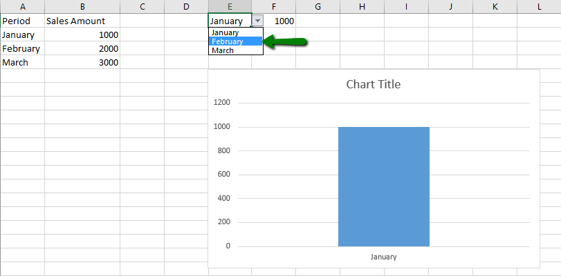
There is nothing wrong with this method, however with one extra step, we can make flipping between these months quicker.

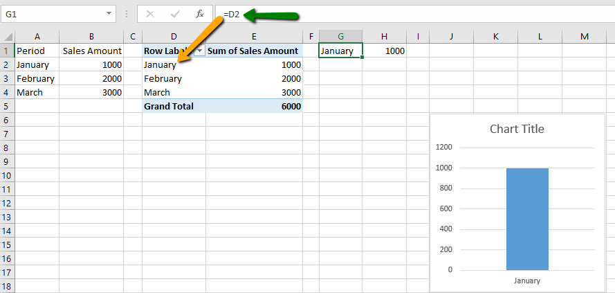
We have introduced a Pivot Table created from the same data range. In cell E1, we have deleted the data list and then referenced the first row of the Pivot Table in cell G1 and H1, which is showing January in this example.

image-2

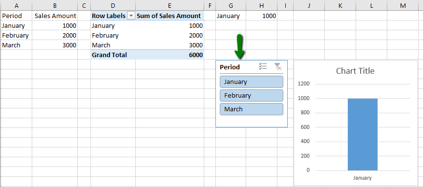
The last step is to simply insert a slicer on that Pivot Table.

To create a slicer, select any cell within the Pivot Table, and then select the Insert Tab, and Slicer under the Filters group.

image-3

Now you can click on the slicer for the month you want to see, rather than having to click on a drop-down list.

image-4

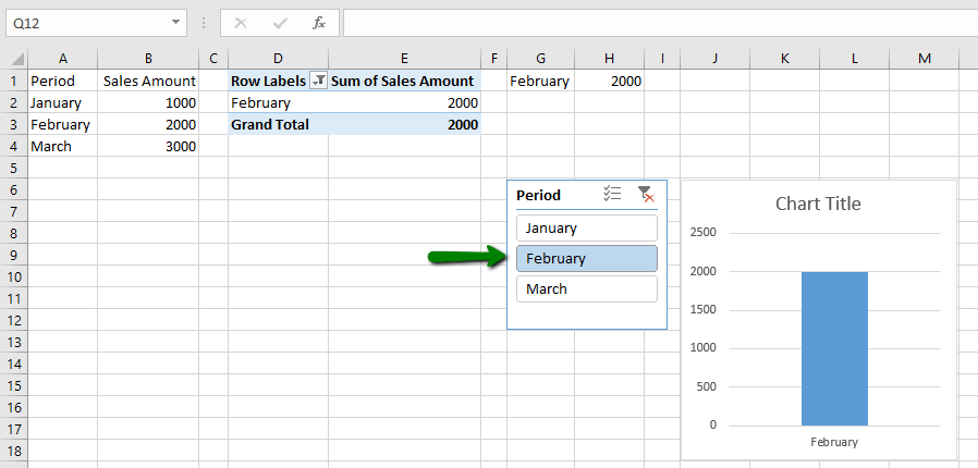
By using this method, time will be saved as the months are easily and quickly selected.

The post How to use a slicer instead of a drop-down list in Excel appeared first on Sage Intelligence.

Source: Excel on Steroids

Post navigation

Learn how to hide rows and columns using Named Ranges
Learn how to extract more than one column of data with a single VLOOKUP formula in Excel

Leave a Reply Cancel reply

Your email address will not be published. Required fields are marked *

Recent Posts

  • Why Working In Excel Works
  • Alchemex Welcomes Velixo 6 For MYOB Advanced
  • Welcome to Velixo Reports Version 4.2
  • Part 3 of 3: Learn how to create a Management Pack in Sage 50cloud Intelligence
  • Part 3 of 3: Create and customize reports easily with the Financial Report Designer

Search

Contact Us

Phone: +61 2 9890 2339
Email: sales@alchemex.com.au
Address: PO Box 212, Deaken West, Canberra, Australia, 2600

Products

  • Intelligence Reporting
  • Velixo Reports

Services

  • Consulting
  • Training
  • Development

About

  • About Us
  • Partners
  • Blog

Support

  • New Ticket
  • Community (Coming Soon)
  • Knowledgebase

Phone: +61 2 9890 2339
Sales: sales@alchemex.com.au
Support: support@alchemex.com.au

Facebook-f Linkedin

© All rights reserved Alchemex Pty Ltd 2020

Made with ❤ by Unfazed Ltd