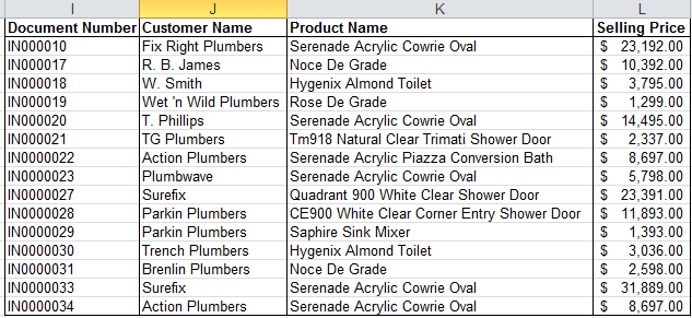
It’s been well over 10 years since I started training Microsoft Excel to corporate clients. During training sessions, delegates would usually ask questions on how they can use Excel to help them become more effective in their work. Last week, a financial manager asked me how she could easily look up more than one field of data from a table with a single VLOOKUP formula.
She wanted to extract the product name, customer name and selling price using one VLOOKUP formula. Her concern was the time it took to extract one field at a time. I therefore decided to write this tip with a view of helping someone save time and increase productivity.
You are welcome to download the workbook to practice.
Applies to: Microsoft Excel 2010 and 2013
1. We are going to extract the product name, customer name and selling price with one VLOOKUP formula. This is the formula we are going to use:
=VLOOKUP(Lookup_value,Table Array,{3,4,6},Range_Lookup).
- Lookup_Value is the common field between the data range and the extraction table.
- Table Array is the source data range.
- The curly brackets represent the position of the fields to be extracted in the source data range. This is not linked to the column letter, but it is the position of the field to be extracted within the table.
- Range_Lookup is either an exact or approximate match
2. Highlight the data range J2 to L2.
3. Type the formula : =VLOOKUP(I2,Data_Source,{3,4,6},0) and press CTRL +SHIFT + ENTER.
- Data_Source is the named range for the data table. Press F3 to display the named ranges and select Data_Source.
- 0 means that an exact match is required.
4. Copy the formula for all three columns.

You can extract more than one column of data with a single VLOOKUP formula, instead of one field at a time. This will help save you time and increase your productivity.
The post Learn how to extract more than one column of data with a single VLOOKUP formula in Excel appeared first on Sage Intelligence.
Source: Excel on Steroids
