If you ever need to split data from one column in your Microsoft Excel worksheet into two or more columns, you can use the LEFT, MID and RIGHT Text functions.
- The LEFT function returns the first character or characters in a text string, based on the number of characters you specify.
- The MID function returns a specific number of characters from a text string, starting at the position you specify.
- The RIGHT function returns the last character or characters in a text string, also based on the number of characters you specify.
The alternative is to use the Text to Columns option, which has been covered in previous tips; however, this option will not work if the source data has formulas such as the VLOOKUP.
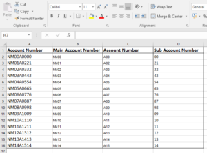
In the example below, we use the LEFT, MID and RIGHT functions to split the System Numbers into Main Account Numbers, Account Numbers and Sub Account Numbers.

You are welcome to download the workbook to practice.
Applies To: Microsoft Excel 2010, 2013 and 2016.
- To extract the Main Account Number using the LEFT function
- Select cell B2.
- Enter the formula: =LEFT(A2,4)
- Copy the formula down.
- To extract the Account Number using the MID function.
- Select cell C2 .
- Enter the formula: =MID(A2,5,3)
- Copy the formula down.
- To extract the Sub Account Number using the RIGHT function.
- Select cell D2 .
- Enter the formula: =RIGHT(A2,2)
- Copy the formula down.
By taking advantage of these easy-to-use functions, you’re able to quickly split data into two or more columns and save time.
The post Quickly split data into two or more columns in Excel appeared first on Sage Intelligence.
Source: Excel on Steroids
