• Products
    • Sage Intelligence Reporting
      • Enrolment
    • Velixo
      • Enrolment
        • Velixo for Acumatica
        • Velixo for Sage Intacct
  • Services
    • Consulting
    • Training
    • Development
  • Support
    • Support Overview
    • Create Support Ticket
    • Book A Session
    • Knowledgebase
  • About
    • About Us
  • Contact
  • Products
    • Sage Intelligence Reporting
      • Enrolment
    • Velixo
      • Enrolment
        • Velixo for Acumatica
        • Velixo for Sage Intacct
  • Services
    • Consulting
    • Training
    • Development
  • Support
    • Support Overview
    • Create Support Ticket
    • Book A Session
    • Knowledgebase
  • About
    • About Us
  • Contact
Quick Support
Book Demo

Using conditional formatting with custom Excel formulas

By admin on February 14, 2018April 19, 2019

Conditional formatting is an effective Microsoft Excel feature that allows you to highlight important information, for example; the ability to find duplicate values within your spreadsheet. You can create your own rule by applying conditional formatting to individual cells or a range of cells.

When you have selected the data you want to format, you can easily change the appearance of how your information is presented to help you easily analyze your data.

You are welcome to download the workbook to practice.

Applies to: Microsoft Excel 2010 and 2013

The format window allows you to change how the information in the cell is presented, without changing the information in the cell itself. However, you can create your own custom rules that go beyond the standard formatting options.

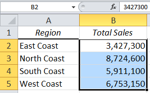
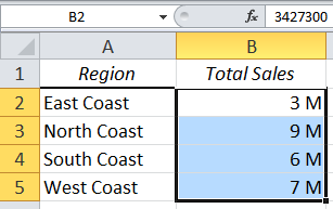
In this example, we have a number of cells containing values in excess of one million. We’ll help you create a rule that will change the appearance of how the values are presented.

1. Open the Excel workbook and select cells B2:B5

Excel on steriods_custom formats_june 2015_2

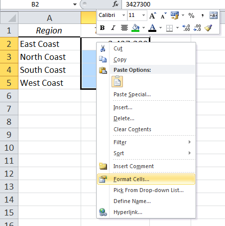
2. Right click on the selected cells and select ‘Format Cells’ (alternatively, use the keyboard shortcut Ctrl + 1)

Excel on steriods_custom formats_june 2015_3

3. In the numbers tab, under the Category group, select Custom

Excel on steriods_custom formats_june 2015_4

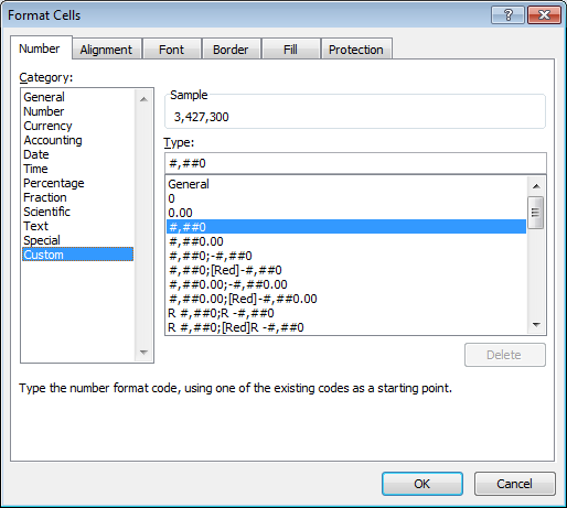
4. In the Type box, delete the current values and enter the following formula

#,###,, “M” and click OK

NB: If you have any difficulty with the above formula, please try the following one: # ###  “M”

Excel on steriods_custom formats_june 2015_5A

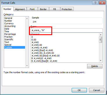
5. The values in the cells are automatically rounded according to their value, along with the letter ‘M’ to signify a million.

Excel on steriods_custom formats_june 2015_6

Now that you have applied your own conditional formatting rule, you can customize your spreadsheets to help you visually analyse data, and identify patterns and trends.

The post Using conditional formatting with custom Excel formulas appeared first on Sage Intelligence.

Source: Excel on Steroids

Post navigation

Troubleshooting your Sage Intelligence errors made easy
Quickly split data into two or more columns in Excel

Leave a Reply Cancel reply

Your email address will not be published. Required fields are marked *

Recent Posts

  • Why Working In Excel Works
  • Alchemex Welcomes Velixo 6 For MYOB Advanced
  • Welcome to Velixo Reports Version 4.2
  • Part 3 of 3: Learn how to create a Management Pack in Sage 50cloud Intelligence
  • Part 3 of 3: Create and customize reports easily with the Financial Report Designer

Search

Contact Us

Phone: +61 2 9890 2339
Email: sales@alchemex.com.au
Address: PO Box 212, Deaken West, Canberra, Australia, 2600

Products

  • Intelligence Reporting
  • Velixo Reports

Services

  • Consulting
  • Training
  • Development

About

  • About Us
  • Partners
  • Blog

Support

  • New Ticket
  • Community (Coming Soon)
  • Knowledgebase

Phone: +61 2 9890 2339
Sales: sales@alchemex.com.au
Support: support@alchemex.com.au

Facebook-f Linkedin

© All rights reserved Alchemex Pty Ltd 2020

Made with ❤ by Unfazed Ltd